Table of Content

• Table of Content
• Linear Clasification
  • Perceptron
  • Stochastic Gradient Descent
    • Loss Functions
    • Gradient Descent
    • Stochastic Gradient Descent
  • Support Vector Machine
    • Maximum Margin Separator
    • Hard-Margin SVM
    • Lagrange Duality
    • Soft-Margin SVM
    • Feature Mapping
    • Kernel Trick
    • Sequential Minimal Optimization

Linear Clasification

Linear classifiers classifies the input features based on the decision hyperplane in the feature space.

Perceptron

The perceptron algorithm is the building block of deep learning. It updates on one data point at each time and moves in the “right” direction based on that point.

Pseudocode

(w/o offset)

k=0, w=0
while not all correctly classified and k < max step:
    for i in 1...n:
        if yi(w•Xi) <= 0: // misclassified
            w = w + yiXi // the Update
            k++

(w/ offset)

k=0, w=0, b=0
while not all correctly classified and k < max step:
    for i in 1...n:
        if yi(w•Xi+b) <= 0: // misclassified
            w = w + yiXi // the Update
            b = b + yi // offset update
            k++

Note: we can convert the w/ offset version to w/o by transforming X to [1, X], then the first resulting weight parameter would be the offset.

Code: algorithm.py - perceptron()

Stochastic Gradient Descent

Perceptron is nice and simple, but it has an important restriction: it only converges on linearly-separable data. To make it work for non-separable data, we need to change the way it approaches the best model.

Loss Functions

A loss function measures the fit of the current model to the training data. For the perceptron algorithm, we want our fitted value to have the same sign as the actual class, so we multiply them together and penalize those with negative products. In another word, the perceptron algorithm uses the following loss function:

A problem with this loss function is that it does not measures the distance between the predicted value and actual class, so 0.1 and 1 will all be seen as good classifications while -0.1 and -1 will all be equally bad.

So another loss function we can use instead is the Hinge Loss, for a fitted value \(\hat{y}\), the Hingle Loss is:

For our linear model, the loss function is defined as:

This loss will penalize any imperfect prediction.

Gradient Descent

The loss function tells us about how bad the current model fits the data. Therefore, we need to know the direction in which moving the parameters will decrease the loss. In mathematics, we use the gradient to measure the “direction.” For Hinge Loss, the gradient of a single data point is:

And the gradient of the whole training data is:

By moving the the weights in the direction of the gradient, we will likely decrease the loss of our model. So the Gradient Descent is defined as:

Pseudocode

k=0, w=0
while criterion not met:
    g = 0
    for i in 1...n:
        if yi(w•xi)<1:
            g = g - yixi/n
    w = w - η*g // the Descent
    k++

η is the step size, or the learning rate.

Stochastic Gradient Descent

The problem with gradient descent is that we need to compute the gradient of each data point in every iteration, which can be slow when the training data is huge. Alternatively, we can update based on a single data point in each iteration, and that is Stochastic Gradient Descent.

Pseudocode

k=0, w=0
while criterion not met:
    for i in 1...n:
        if yi(w•xi)<1:
            w = w + η*yixi // the Descent
            k++

Code: algorithm.py - SGD() / GD()

Support Vector Machine

As mentioned before, in linear classification problems we want to find a hyperplane that separates training data well. But there can be infinitely many hyperplanes that separate the data, we need to have additional measures to select the best ones.

Maximum Margin Separator

Consider the following example:

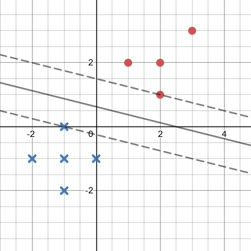
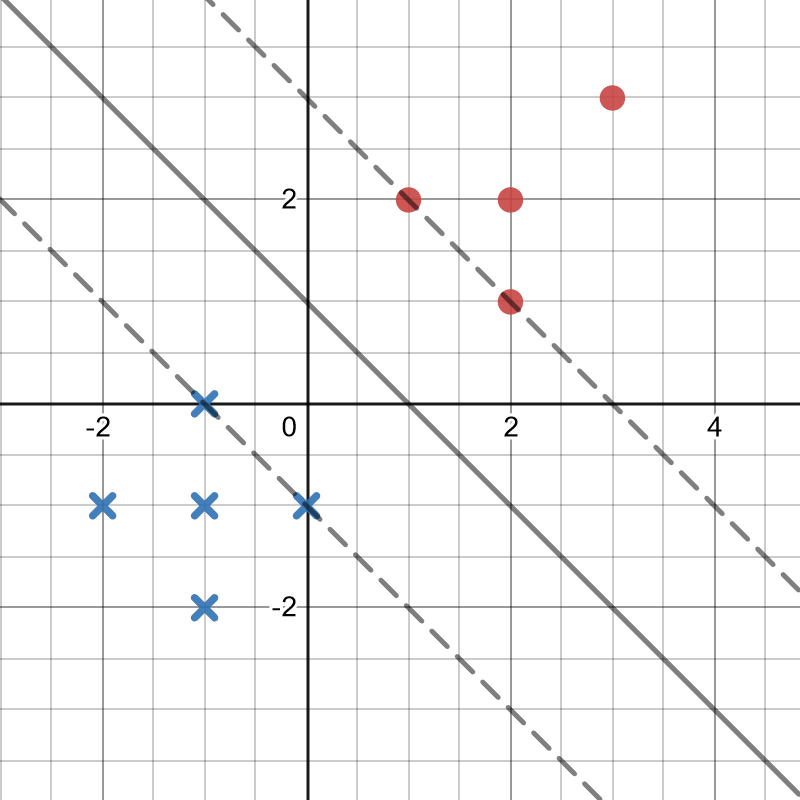
The solid lines on each figure represents a classification boundary that separates the two training classes. They both perfectly classify the training data, but which one is better? We would consider the right one better because it maximizes the “margins” between the separator and the training data.
So while using the Hinge Loss may produce either of the above models, maximizing the margin will give us the better model. In another word, we want to maximize the distance from the closest point to the separating hyperplane:

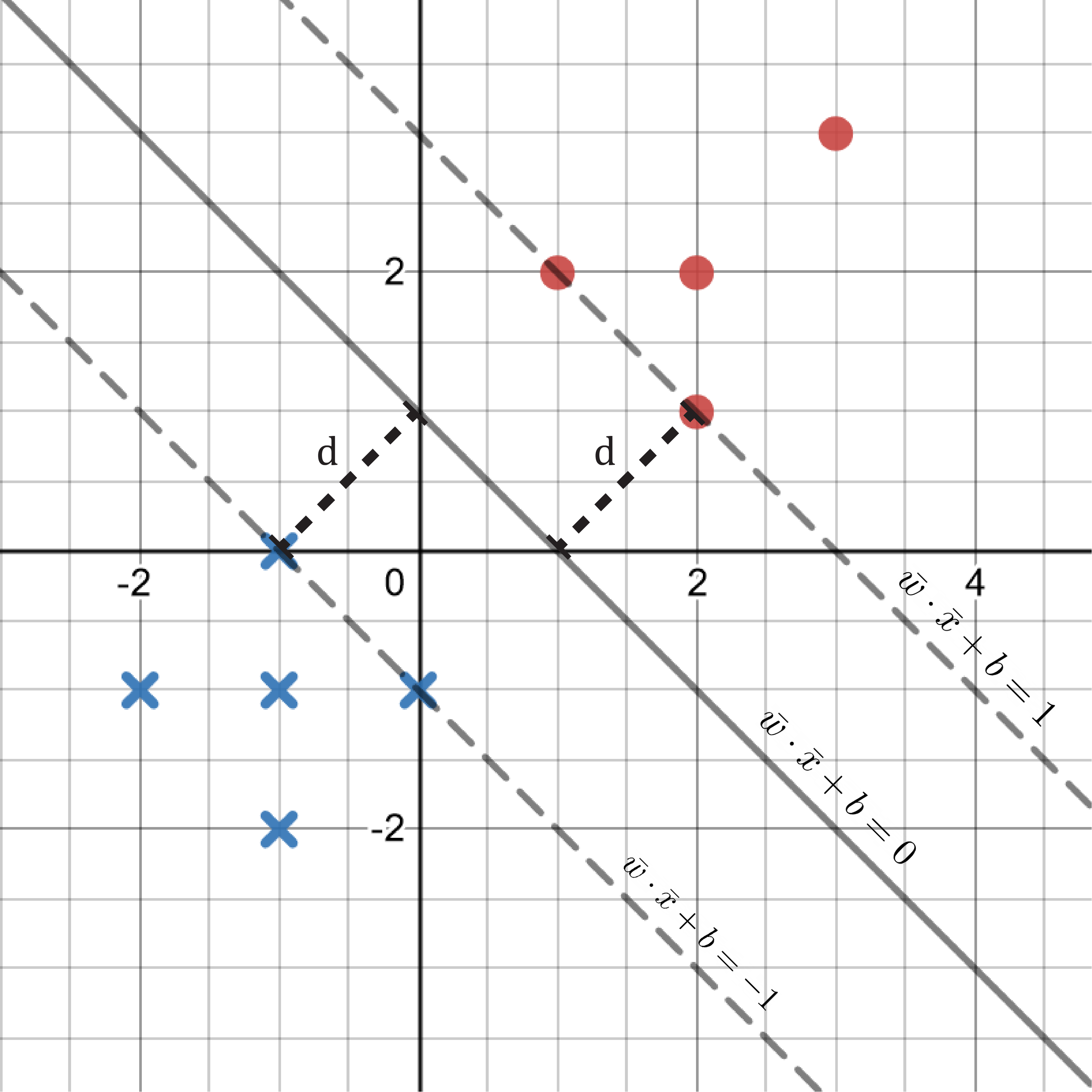
If we look at the two margine lines, they are actually the decision lines \(\mathbf{w}\cdot\mathbf{x}+b=1\) and \(\mathbf{w}\cdot\mathbf{x}+b=-1\) beecause they are right on the border of being penalized. So we can calculate the margin as the distance between the positive margin line and the decision boundary:

And we want our model to maximize the margin:

Hard-Margin SVM

We can now formulate our problem as a constrained optimization. For computation purpose, we transform the maximization into a minimization problem:

Lagrange Duality

For a constrained optimization problem \(\min_{\textbf{θ}}{f(\textbf{θ})}\) subject to \(\eta\) constraints \(h_i(\textbf{θ})\leq 0,\forall i\in{1,…,n}\), we can combine the objective function with the contraints using the Lagrange multipliers \(\lambda_1,…,\lambda_n\geq0\).

From this formation, we observe that if a model satifies all the constraints, \(f(\textbf{θ})\geq L(\textbf{θ},\textbf{λ})\), so minimizing \(f\) is the same as minimizing the maximum of \(L\), that is:

This is called the primal formulation. And we have dual formulation:

The dual provides a lower bound for the primal solution, so there is a duality gap between the two formulations. The gap is 0 if the Karush–Kuhn–Tucker (KKT) conditions are satisfied:

For our hard-margin SVM, the gap is 0. The Lagrangian function is:

To satisfy the stationarity conditions, we need the gradient with respect to \(\mathbf{w}\) and \(b\) to be 0:

Using the dual formation, our problem become:

According to the complementary slackness condition \(\alpha^\ast_i(1-y^{(i)}(\mathbf{w}^\ast\cdot\mathbf{x}^{(i)}+b^\ast))=0\):

We can also compute the intercept \(b\) using the support vectors:

Soft-Margin SVM

However the hard-margin SVM above has limitations. If the data is not linearly separable, the SVM algorithm may not work. Consider the following example:

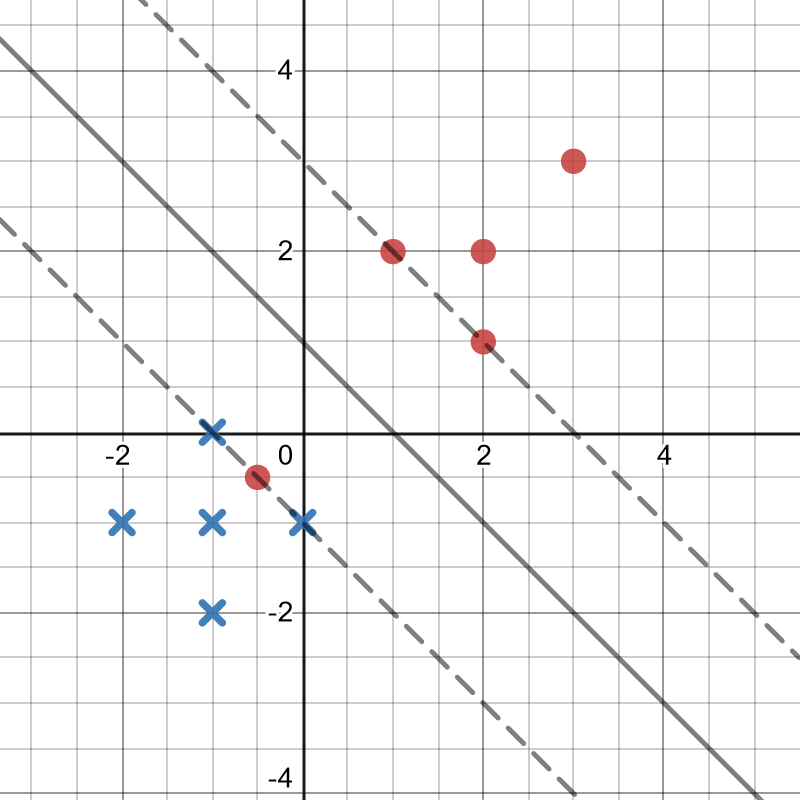
If we use hard-margin SVM, the fitted model will be highly affected by the single outlier red point. But if we allow some misclassification by adding in the slack variables, the final model may be more robust. The setup for a soft-margin SVM is:

The Lagrangian is:

We first find the gradient with respect to \(\mathbf{w}\), \(b\), \(\textbf{ξ}\), and we need them to be 0:

And the dual formulation is:

We can see that soft-margin SVM has a same dual formulation as the hard-margin SVM. And now, the condition for optimum are \(\alpha_i^\ast(1-\xi_i^\ast y^{(i)}(\mathbf{w}^\ast\cdot\mathbf{x}^{(i)}+b^\ast))=0\) AND \(\beta_i^\ast(-\xi_i^\ast)=0\), so combining them together:

An observation that can be drawn from this result is that \(C\) is a hyperparameter that controls the “softness” of our SVM model. If \(C\) is big enough, the soft-margin SVM will become a hard-margin one.

Feature Mapping

Soft-margin SVM seems to provide a decent approach to non-linearly separable data, but it only works well when there are a few “noisy” data. When the boundary between categories is inherently non-linear, it is not reasonable to use a soft-margin SVM. For example:

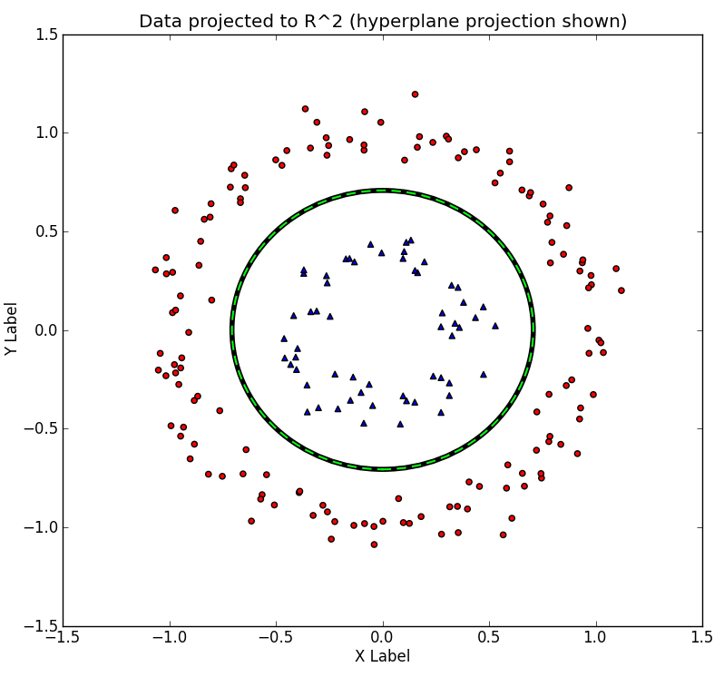
We cannot find a separating hyperplane, so the SVMs we have discussed will not work as expected. However, if we jump out of the 2-dimensional space, we can find hyperplanes that can separate the data:

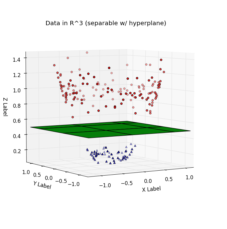
The way we convert the lower-dimensional coordinates into higher ones is called a feature mapping.

Kernel Trick

Assume we have a feature mapping \(\phi(\cdot):\mathcal{X}\rightarrow\mathcal{F}\) and we fit this mapped data using SVM, then the objective function would be:

One problem with this setup is that the computation can be slow because we need to 1) map the features to higher dimension, 2) compute the inner products between each pair of mapped features. Also, note that predicting the response for a new data point is:

We can see that only the inner product of the mappings are needed in training or evaluation. So instead of computing the mapping, we would like to compute the inner products of the mapped features directly. Therefore, we introduce the kernel function:

Then we can rewrite the objective function as:

According to Mercer’s Theorem, a kernel function is valid if and only if its Gram matrix must be positive semi-definite. Below are some properties of kernel functions, let \(K_1,K_2:\mathcal{X}\times\mathcal{X}\rightarrow\mathbb{R}\) be two valid kernels of feature mapping \(\phi_1:\mathcal{X}\rightarrow\mathbb{R}^{M_1},\phi_2:\mathcal{X}\rightarrow\mathbb{R}^{M_2}\), then the following kernels and feature maps \(K:\mathcal{X}\times\mathcal{X}\rightarrow\mathbb{R},\phi:\mathcal{X}\rightarrow\mathcal{F}\) are valid (\(\phi\) is not unique):

Using these properties, we can come up with some useful kernel functions:

While the linear and polynomial kernels may be obvious (use the addition and product rule), the RBF kernel can be hard to interpret:

Now this looks like the second transformation above, we would like to prove the middle term a kernel. We will use Taylor expansion:

So the middle term is in fact an infinite positive-weighted-sum of polynomial kernels, which is also a valid kernel. And we can tell that the feature mapping of a RBF kernel will have infinite dimensions, so it proves the importance of a kernel function as calculating the mapped features can be impossible.

Sequential Minimal Optimization

Reference: John C. Platt, Sequential Minimal Optimization: A Fast Algorithm for Training Support Vector Machines

Now the only thing we need is to pick the multipliers to optimize the objective function. In another word, we are solving this Quadratic Programming problem:

The main idea of the Sequential Minimal Optimization (SMO) algorithm is to optimize only a pair of multipliers each time. It works as following:

Pseudocode:

α=0, b=0 
while not all α satisfies KKT conditions:
    pick αi, αj using some heuristics
    optimize αi, αj
    update b

The optimization for each pair can be represented as (\(\delta\) is the sum of the rest terms):

Now we can substitute \(\alpha_j\) for \(\alpha_i\):

To optimize, we take the partial derivative w/ respect to \(\alpha_j\):

If we look at the two sum terms \(S_i\), \(S_j\):

We want to derive the optimized \(\alpha_j\) by making the derivative to 0, assume we are currently at step \(k\):

Therefore, we are able to use the residual values and the kernel function to calculate the optimized \(\alpha_j\), and thus \(\alpha_i\) and \(b\). But before that, we need to check the constraints \(0\leq\alpha_i^{k+1},\alpha_j^{k+1}\leq C\). Since \(\alpha_i^{k+1}y^{(i)}+\alpha_j^{k+1}y^{(j)}=\alpha_i^{k}y^{(i)}+\alpha_j^{k}y^{(j)}=\zeta\):

Therefore, we can get the lower and upper bounds of \(\alpha_j^{k+1}\), \(L^{k+1}\) and \(H^{k+1}\), based on the value of \(y^{(i)},y^{(j)}\), and “clip” the value of \(\alpha_j^{k+1}\):

And we can get \(\alpha_i^{k+1}\):

Now we want to get the offset value \(b^{k+1}\) by using the support vectors:

If \(\alpha_i^{k+1}\) is on the margin, we will set \(b^{k+1}=b_i^{k+1}\); if \(\alpha_j^{k+1}\) is on the margin, \(b^{k+1}=b_j^{k+1}\); if they are both on the margin, \(b^{k+1}=b_i^{k+1}=b_j^{k+1}\). But if none of them is on the margin, the SMO algorithm chooses the average value \((b^{k+1}=b_i^{k+1}+b_j^{k+1})/2\).

Now we are able to optimize any pair of multipliers, \(\alpha_i^{k+1}\) and \(\alpha_j^{k+1}\), and get the updated offset value, \(b^{k+1}\). But we have not talked about the mechanism of choosing the pair, \(\alpha_i^{k}, \alpha_j^{k}\). In Platt’s original paper, two heuristics are used for \(\alpha_i\) and \(\alpha_j\) respectively:

• For \(\alpha_i\):

  If all \(\alpha=0\) or \(C\), choose \(\alpha_i\) that violates the KKT conditions
  Otherwise choose \(0<\alpha_i< C\) that violates the KKT conditions
  

• For \(\alpha_j\):

  Choose \(\alpha_j\) that maximize \(|E_i-E_j|\). The algorithm will keep track of \(E_k\) for all \(0<\alpha_k< C\)

Note we only need to check the complementary slackness conditions here because the other conditions are enforced by the SMO algorithm. A full pseudocode can be found in Platt’s paper.

Alternatively, we can give up the heuristics and instead randomly select \(\alpha_j\) for each \(\alpha_i\). This Simplified SMO is much easier to implement:

Pseudocode:

α=0, b=0
tol=1e-3, ε=1e-5
iter=0
while iter<max_iter: // stop when max_iter pass of no updates
    k = 0 // number of α changed
    for i in 1...n:
        Ei=f(xi)-yi
        if (yiEi<-tol and αi<C) or 
                (yiEi>tol and αi>0): // KKT condition
            random j!=i
            Ej=f(xj)-yj
            compute L, H
            if L==H:
                continue
            η=K(xi,xi)+K(xj,xj)-2K(xi,xj)
            if η>=0:
                continue
            αj'=αj+yj(Ei-Ej)/η
            clip αj' with L, H
            if |αj-αj'|<ε:
                continue
            αi'=αi+yiyj(αj-αj')
            compute bi, bj
            if 0<αi'<C:
                b'=bi
            elif 0<αj'<C:
                b'=bj
            else:
                b'=(bi+bj)/2
            αi=αi', αj=αj', b=b'
            k++
    if k==0:
        iter+=1 // can't optimize w/ αi
    else:
        iter=0

Code: _svm.py